
Introduction
The dramatic increase in multi-color fluorescence microscopy applications witnessed over the past decade is due, in part, to the significant advances in instrument and detector design as well as the introduction of a vast array of new fluorophores, including synthetics and quantum dots. In addition, live-cell imaging has been revolutionized by the introduction of ever increasingly useful genetically-encoded fluorescent proteins spanning the entire visible spectral region. Among the primary advantages of using multiple fluorescent labels in fixed and living cells and tissues is the ability to observe the spatial relationship and temporal dynamics of subcellular constituents, and to monitor potential molecular interactions between differently labeled entities. A number of advanced microscopy techniques have been applied using multi-color fluorescence labeling, including fluorescence recovery after photobleaching (FRAP), fluorescence correlation spectroscopy (FCS), fluorescence (or Förster) resonance energy transfer (FRET), fluorescence in situ hybridization (FISH), and fluorescence lifetime imaging (FLIM). Many of these methods benefit significantly from the ability to use specifically targeted fluorescent proteins in live-cell imaging experiments.
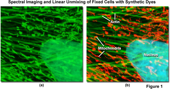
Spectral imaging combined with linear unmixing is a highly useful technique (see Figure 1) that can be used in combination with other advanced imaging modalities to untangle fluorescence spectral overlap artifacts in cells and tissues labeled with synthetic fluorophores that would be otherwise difficult to separate. Illustrated in Figure 1 is an Indian Muntjac fibroblast cell stained with a combination of SYTOX Green (nucleus), Alexa Fluor 488 conjugated to phalloidin (filamentous actin network), and Oregon Green 514 conjugated to goat anti-mouse primary antibodies (targeting mitochondria). These dyes have emission maxima at 523, 518, and 528 nanometers, respectively, and each appears green to the eye when viewed in widefield fluorescence using a standard FITC cube (Figure 1(a); imaged in confocal mode with a 488-nanometer argon-ion laser). Using laser scanning confocal microscopy coupled with a spectral imaging detector, the entire spectrum of fluorophores in the specimen was first gathered (Figure 1(a)), and then linearly unmixed and assigned pseudocolors (Figure 1(b); nucleus, cyan; actin, green; mitochondria, red) to more clearly delineate the relative proximity of the various structures.
Shortly after enhanced green fluorescent protein (EGFP) was introduced as a viable probe for live-cell imaging in the mid-1990s, investigators began to fuse the purified DNA sequence to that of a wide variety of endogenous proteins having highly specific intracellular targets. The resulting genetically-expressed chimeras are able to serve as molecular beacons to enable tracking of virtually any protein of interest in living cells. Fluorescence imaging of EGFP alone is relatively straightforward and can be readily conducted using a single longpass emission filter that covers the entire green-to-red spectral region (approximately 520 to 650 nanometers). For abundant targets, a high level of signal can be captured with virtually any digital camera system using this configuration. However, with the emergence of new fluorescent proteins in the lower wavelength emission regions (blue and cyan), as well as those emitting at longer wavelengths (yellow, orange, red, and far red), the use of bandpass emission filters becomes necessary in order to segregate the emission of closely overlapping spectra in experiments using two or more fluorescent proteins.
Although recent advances in synthetic fluorophore technology and the development of biological quantum dot conjugates promises to ultimately yield tremendous flexibility in labeling of fixed cells and tissues, live-cell imaging techniques currently rely heavily on the use of fluorescent proteins fused to target peptides and proteins that label specific proteins and subcellular organelles. However, even though a wide variety of new fluorescent protein color variants have become available in the past few years, the number of proteins that can be simultaneously imaged in multi-color investigations is limited by the broad, overlapping spectral profiles of these fluorophores. For example, several of the most useful variants, including enhanced cyan, green, and yellow fluorescent protein (ECFP, EGFP, and EYFP), perform superbly in fusions and are very useful when imaged alone. Unfortunately, these probes have strongly overlapping emission spectra that are virtually impossible to separate into specific channels during colocalization experiments using traditional interference filters. In most cases, narrow bandwidth emission filters must be utilized to discriminate between two or more fluorescent proteins, which results in the significant loss of otherwise useful signal. In live-cell imaging experiments, however, it is necessary to gather as much signal as possible to minimize the required expression level of fluorescent proteins and to reduce the intensity of excitation light in order to avoid phototoxicity.
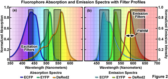
The emission profile of a typical fluorophore is usually non-symmetrical (with the exception of quantum dots) such that the slope of the curve is far steeper for wavelengths shorter than the maximum (peak) and much broader for longer wavelengths past the peak, which contain most of the total fluorescence emission, as illustrated in Figure 2(b). The full width at half maximum (FWHM; the measure of bandwidth size of a spectral profile at 50-percent of the maximum intensity) of most synthetic fluorophores used in fluorescence imaging ranges from 20 nanometers to over 60 nanometers, whereas that of fluorescent proteins averages between 40 and 150 nanometers. Given that the visible light spectrum spans a wavelength range of approximately 300 nanometers (400 to 700 nanometers), it is apparent that only a limited number of synthetic fluorophores or fluorescent proteins can be simultaneously imaged in this region without incurring bleed-through artifacts due to significant spectral overlap. Note that bleed-through is often referred to as crosstalk in the scientific literature; however, the two terms are considered synonymous. As the desire to conduct experiments using specimens having more than two fluorescent labels increases, the ability to quantitatively assess resulting datasets is often compromised by a number of factors, including the inability to limit emission to a single detection channel. Thus, the unambiguous identification of specific fluorescence information is not always possible, particularly when there exists a mixture of strong and weak signals or if the choice of probes is limited, as is often the case for fluorescent proteins.
Imaging Multiple Fluorescent Probes
When imaging multiple fluorophores in widefield fluorescence microscopy, bleed-through artifacts can often be overcome by the judicious choice of filter combinations. In addition to considering the emission spectral overlap of fluorophores, cross-excitation due to overlapping absorption bands must also be addressed. Excitation filters having sufficient bandwidth to efficiently excite a single fluorophore should be combined with emission filters that allow the highest level of signal to be gathered (see Figure 2). Due to the fact that excitation efficiency of a fluorophore decreases rapidly at wavelengths removed from the peak (the degree of which depends upon the FWHM), several spectrally distinct fluorophores can be sequentially excited using relatively narrow bandpass filters centered near their peak absorption wavelengths. Thus, if the filter excitation regions and bandwidths are properly chosen, two fluorophores having significant overlap in their emission profiles may not generate bleed-through during imaging. This strategy is highly effective with standard fluorophores, such as DAPI (4',6-diamidino-2-phenylindole), fluorescein, rhodamine, and Cy5, when the acquisition is sequential (in effect, only one fluorophore is excited at a time) and narrow bandpass emission filters are employed. Unfortunately, up to 50 percent or more of the available fluorescence emission is rejected and the total acquisition time is increased, which can be a significant problem with dynamic live-cell imaging due to the fact that cellular movement between channel captures often introduces registration errors when two or three channels must be combined into a multicolor image. Furthermore, the choice of useful fluorescent proteins in widefield fluorescence microscopy is still limited, and those that perform the best in live-cell imaging experiments have considerable spectral overlap that cannot be completely separated with standard filters.
In laser scanning confocal microscopy, the situation is similar, but laser illumination is used as the excitation source instead of bandpass interference filters coupled to a broadband light source. Still, a dichromatic mirror is used to separate excitation illumination from the emission signal that is sent to a photomultiplier tube, rather than a CCD camera system. Unlike widefield fluorescence, however, laser illumination can be carefully controlled during the scan cycle to reduce or avoid bleed-through when there is overlap in the excitation spectra of two fluorophores. Termed multitracking, fast switching between laser lines using an acousto-optic tunable filter (AOTF) or similar device can enable separate excitation (and the subsequent gathering of fluorescence emission) of each fluorophore, either line-by-line or for an entire image frame. For example, when imaging EGFP and mCherry (a red fluorescent protein), the 488-nanometer argon-ion laser spectral line might be used to excite EGFP across a single line of the frame, collecting fluorescence emission as it goes along. On the return (along the same scan line) the 561-nanometer laser spectral line is then used to excite mCherry and gather emission. Such a process avoids exciting both fluorescent proteins simultaneously and can significantly reduce emission spectral bleed-through. Unfortunately, when using two overlapping fluorescent proteins, such as EGFP and EYFP, the 488-nanometer laser line will excite both fluorophores simultaneously, requiring a different solution.
For the analysis of quantitative experiments, including FRET and colocalization, the presence of spectral bleed-through and autofluorescence introduces complications that often require correction. In some cases, ratiometric techniques can be utilized to quantify the fluorescence of each of the fluorophores in a specimen or to assess changes in a ratiometric indicator. For instance, it is possible to estimate the amount of bleed-through that is likely to occur when two fluorophores are imaged together simply by measuring the level of bleed-through that is present using specimens containing only a single label. In practice, usually two excitation wavelengths coupled with two different emission detection channels are used to determine the signal level obtained in the separate channels when each fluorophore is excited. After the signal ratio is determined for each probe, the correction value can be applied to the experimental raw data. Once again, however, for fluorescent probes having closely overlapping excitation and emission spectra (as is common for FRET donors and acceptors), co-excitation of both fluorophores is generally a problem and it becomes difficult or even impossible to separate emission using either narrow bandpass filters or laser multitracking. Furthermore, differences in fluorescent protein expression levels, background noise, autofluorescence, mismatched detector response, and complications arising from the use of more than two labels (along with a variety of other factors), can combine to make ratiometric correction techniques cumbersome or useless in separating emission signals.
Spectral Imaging
When experimental conditions permit, the thoughtful selection of fluorescent labels, laser multitracking strategies, filter set characteristics, and control specimen correction factors can combine to yield excellent results. In the real world, however, situations often arise where the choice of experimental parameters is limited and the use of fluorescent probes lacking in significant spectral overlap is not feasible. Such a scenario is often encountered when attempting to conduct multiple labeling investigations with fluorescent proteins. Experiments are also subject to artifacts arising from natural autofluorescence or fluorescence induced by the use of fixatives or DNA transfection reagents, which can span several detection channels. In these cases, a technique known as spectral imaging coupled with image analysis using linear unmixing can be employed to segregate mixed fluorescent signals and more clearly resolve the spatial contribution of each fluorophore (often referred to as emission fingerprinting). Microscopes are now available that have been specifically designed to accommodate spectral imaging and, although the technique bestows significant advantages, it also increases the complexity and purchase price of the instrument.
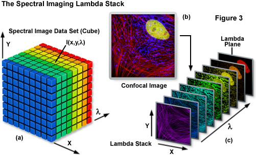
Spectral imaging merges the two well-established technologies of spectroscopy and imaging to produce a tool that has proven useful in a variety of disciplines that rely on various forms of optical microscopy. The methodology has been extensively applied to visualize the chemical composition of materials ranging from enzymes involved in biomolecular interactions to the formation of stars. Unlike a typical image, which is acquired over the entire wavelength response band of the detector, a spectral image requires the creation of a three-dimensional data set that contains a collection of images of the same viewfield captured at different wavelengths or wavebands. In effect, the spectral image provides a complete spectrum of the specimen at every pixel location (noted as I(x,y,λ); see Figure 3) throughout the lateral dimensions. Thus, a spectral image stack can be considered as either a collection of images, each of which is measured at a specific wavelength or over a narrow band of wavelengths, or as a collection of different wavelengths at each pixel location.
Remote sensing analysis has for many years employed spectral imaging techniques to investigate how light waves from the sun are reflected and scattered from the Earth's surface and within the atmosphere. Careful examination of the spectral frequencies present in satellite image datasets allows the different objects, landscapes, and terrains to be identified and characterized. In effect, by measuring intensity variations as a function of wavelength in order to correlate pixels with matching spectral information, a number of details can be revealed that are missing from single images captured when all of the light from the visible spectrum is used. These geological spectra are far more complex than those obtained in biology due to the fact that the number of spectral classes is significantly larger than the number of fluorescent probes that can be practically applied in a biological investigation. However, the overall spectral signature of multiband satellite images is analogous to that obtained from a convolved spectrum of multiple fluorophores in a living cell expressing several fluorescent proteins or a pathological thin section stained with absorbing synthetic dyes. Over the past several years, satellite imaging approaches have been applied with increasing success in the examination of biological samples to solve problems related to spectral karyotyping, resonance energy transfer, colocalization, stained tissue analysis, and the elimination of autofluorescence. The spectral information gathered from these biological specimens is used to determine the location of specific dyes and fluorophores, and often yields information about interactions between them.
The Lambda Stack
The spectral image stack (I(x,y,λ)) discussed above is commonly referred to in the scientific literature as a lambda stack, image cube, or spectral cube having wavelength bands generally ranging from 2 to 10 nanometers and image dimensions up to a million pixels (see Figure 3), depending upon the instrument configuration. For all practical purposes in fluorescence microscopy, a lambda stack can be considered analogous to a time-lapse series or optical section z-stack gathered by a widefield deconvolution or confocal microscope. For a qualitative assessment of the lambda stack, a region of interest in the x-y dimension (lateral focal plane) can be examined along the wavelength axis to determine how pixel intensity and/or color changes due to signal level variations at different emission bands (λ planes; Figure 3(c)). In other words, the emission spectrum of a particular fluorophore can be determined by plotting the pixel intensity versus the center wavelength of each emission band. The accuracy of the emission spectra obtained by this technique depends largely on the number of images gathered at distinct wavelength bandwidths, the bandwidth size (shorter bandwidths yield more accurate spectra), specimen quality, and the instrument detector sensitivity. In confocal microscopes that use separate pinholes for each detector, wavelength-dependent variations can occur in optical section thickness for the different spectral channels. However, most modern instruments are designed with a single pinhole for all detectors and, in any event, probes with highly overlapping spectra are usually very similar in spectral range.
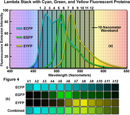
As an example of a typical confocal fluorescence lambda stack acquired at 512 x 512 pixels, consider a specimen labeled with three spectrally overlapping fluorescent proteins, ECFP (emission maximum at 475 nanometers), EGFP (emission maximum at 509 nanometers) and EYFP (emission maximum at 527 nanometers), which has been scanned in twelve 10-nanometer wavebands from 460 to 580 nanometers (see Figure 4(a)). The first image of the lambda stack will reveal the spectral signature (emission fingerprint) of the specimen in the emission range of 460 to 470 nanometers, including a moderate level of signal from the short-wavelength tail of the ECFP emission spectrum but without significant fluorescence emission from EGFP or EYFP (which do not exhibit any detectable emission until about 480 nanometers). In the 510 to 520 nanometer band (near the EGFP peak emission), the contribution of ECFP, EGFP, and EYFP will be approximately 60 percent, 70 percent, and 30 percent, respectively. Likewise, the 520 to 530 nanometer band (near the EYFP peak) will include contributions from ECFP and EGFP of approximately 40 percent and from EYFP of approximately 60 percent. Finally, the last waveband in the series will span the region of 570 to 580 nanometers and includes a significantly greater contribution from the long-wavelength emission tail of EYFP than from either ECFP or EGFP. In this representative lambda stack, the distribution of the mixed emission signal across the waveband channels can be linearly unmixed (see below and Figure 4(b)) using the individual fluorescent protein emission fingerprints to clearly separate the contribution from each probe.
In order to acquire a lambda stack, the instrumentation must be capable of capturing successive images of a particular specimen at different excitation or emission bandwidths. A variety of different techniques have been applied to generate lambda stacks in both widefield and confocal microscopy. The simplest method is termed wavelength-scan and gathers the images one wavelength (or waveband) at a time, usually with a collection of interchangeable narrow bandpass interference filters augmented by a combination of shortpass and longpass filters having particularly sharp cut-off wavelengths. In this configuration, the bandpass size of the filters determines the number of wavelengths included in each lambda scan. The filters are positioned in front of the photomultiplier (or a CCD camera) and a filter wheel rotates a bandpass or pair of longpass-shortpass filters into the optical path to acquire wavelength bands of equal bandwidth. Although using a large number of filters offers greater flexibility in the available bandwidths and spectral range for gathering lambda stacks, this technique is practical only in situations where a limited number of wavebands are required. A significant drawback to the filter-based approach is the requirement for repetitive scanning of the specimen, which is necessary in order to gather successive images at each wavelength increment. The process is inherently slow (not useful for live-cell imaging) and is further hampered by increased photobleaching that occurs during extended periods of acquisition.
An alternative mechanism for obtaining wavelength-scan lambda stacks is to utilize one of several variable-filter techniques, including variable spectrum interference filters and tunable optical filters. Tunable filters acquire a lambda stack by capturing a series of images at each wavelength band and have the flexibility to select a large number of bands. A circular variable filter operates by transmitting a narrow waveband of excitation or emission light that can be fine-tuned by rotating the filter in the light path. This method has not been applied in commercial instruments and suffers from the artifact that images contain a superimposed spectral gradient. A superior alternative involves the application of acousto-optical tunable filters (AOTFs) or liquid crystal tunable filters (LCTFs) either between the illumination source and specimen (for broadband sources) or between the specimen and the detector. The latter configuration often suffers from the poor transmission efficiency in some filter designs (due to polarization and scattering artifacts), which can significantly reduce signal-to-noise. LCTF filters operate by transmitting a narrow band of wavelengths (down to a single nanometer) when a voltage is applied to a birefringent liquid crystal mounted between two linear polarizers. In general, several stages are necessary to achieve high resolution, which reduces the total transmission of light through the filter. AOTF filters are composed of specialized acoustic-sensitive crystals (such as tellurium dioxide) that can be tuned to transmit specific wavelength bands through the application of orthogonal acoustic waves. Depending upon the applied acoustic frequency (with switching speeds measured in microseconds), the crystal deforms to simulate a diffraction grating with a specific period. AOTF filters have drawbacks that have limited their use on the emission side in fluorescence microscopy, including poor light throughput as well as image blur and shift.
Evolution of spectral imaging instrumentation targeted at live-cell studies has pushed the development of rapid lambda stack acquisition strategies that limit the number of times the specimen is exposed to excitation illumination. In this regard, the entire spectrum of an image is acquired using spatial-scan techniques, which scan the specimen either point-by-point or line-by-line. Spatial approaches rely on dispersion of fluorescence emission using either a prism or diffraction grating and are usually implemented in laser scanning confocal microscopes (see Figure 5). When the emission light is separated into component colors by passing through a prism, individual channels (photomultipliers) can gather selected portions of the light spectrum using variable-width slits and mirrored optical components (Figure 5(b)). In commercial implementations, the slit width is adjustable to select the desired bandpass size of light entering the first detector. Additionally, the surface of the slit is mirrored to reflect light not entering the slit to a second detector/slit combination. Such instrument designs are capable of implementing multiple detection channels, so that there are no physical gaps in the light spectrum and the number of images in a lambda stack (regardless of the bandwidth) is limited only by the number of photomultipliers.
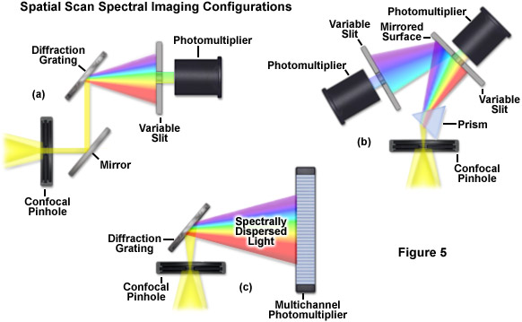
A more versatile configuration, which greatly enhances lambda stack acquisition speed, employs a unique multichannel photomultiplier to gather bands of fluorescence emission light that have been separated into component colors using a diffraction grating (Figure 5(c)). By employing a linear array of detection channels, multiple emission bands are imaged in parallel, thus enabling a selected spectral region to be obtained in a single scan across the specimen (minimizing phototoxicity). In commercial microscope implementations, the diffraction grating disperses the emitted fluorescence, which is then directed onto an array of precisely defined bandwidth channels in a specialized multi-anode photomultiplier (either 9.7-nanometer or 10.7-nanometer channels in a 32 channel detector) to generate a separate image from each channel. As a result, in some microscopes, eight images in a lambda stack can be simultaneously produced by a single scan spanning a spectral region that is dependent upon the product of the combined channel bandwidths. More advanced spectral imaging confocal microscopes can acquire 32 images simultaneously. Several instruments based on diffraction grating separation also employ an efficiency enhancement system that is designed to decrease wavelength losses at the spectral grating. In situations where a larger spectral width is required, additional scans can be added or adjacent channels can be combined (binned) to double, triple, or quadruple the width of the detection band.
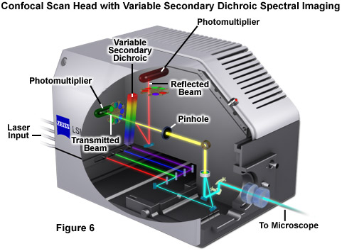
Perhaps the simplest configuration using a laser scanning confocal microscope for spectral imaging couples a diffraction grating with an adjustable slit that can be mechanically translated across the input window of the photomultiplier detector (Figure 5(a)). Fluorescence emission passing through the pinhole is reflected onto the diffraction grating surface using a dichromatic mirror. The spectrally separated light is then projected through the slit and into the photomultiplier. The spectral bandwidth can be modulated by increasing or decreasing the slit size and the wavelength region presented to the photomultiplier is determined by the position of the slit in relation to the dispersed light from the grating. Another innovative, yet simple, design incorporates an interference filter device termed a variable secondary dichroic (VSD), which serves as a beamsplitter to direct selected wavelength bands into separate photomultiplier detectors (see Figure 6). The vertical position of the VSD unit with respect to the emission beam in the confocal optical train determines the wavelength band that is transmitted to the first of two photomultipliers. The second photomultiplier receives light of longer wavelength that is reflected from the surface of the VSD. Wavelength selection using the VSD is easily achieved simply by shifting the position of this dichromatic beamsplitter element.
Widefield microscopes can be adapted for spectral imaging using a technique known as Fourier transform imaging spectroscopy by coupling an interferometer to a fluorescence microscope. In this configuration, light gathered by the objective is directed to the interferometer, which splits it into two independent beams and simultaneously introduces a minute optical path difference (OPD) with a slight time delay between the beams. After passing through the microscope optical train and specimen, the beams are subsequently recombined to create an interference pattern that is projected onto the digital camera (CCD) detector. The resulting intensity pattern of varying OPDs at each pixel is termed an interferogram, which is specific to the spectral content of the specimen. The image stack can then be treated with a fast Fourier transform (FFT) algorithm to determine the profiles and spatial locations of the contributing spectra. Among the advantages of this methodology are that no filters are required to separate emission because the spectrum is measured using the interference of light, and the intensity at each wavelength is collected for each image captured during the process. Additionally, the spectral resolution is determined by acquisition parameters and can be changed without modifications to the hardware configuration. On the downside, the full spectrum must be collected for each image even when only a limited region is required for the experiment. Fourier transform spectroscopy is widely employed for spectral karyotyping and has also been applied with linear unmixing to separate emission from colocalized fluorescent probes.
As temporal acquisition speeds steadily increase to capture exceedingly fast events in live-cell imaging, the ability to simultaneously measure spectral parameters in large spatial dimensions is necessarily compromised by the limits on detector sensitivity. Generally, these limitations can be overcome by selecting a smaller region of interest and restricting the number of wavelength bands that are captured. A similar approach has been successful in flow cytometry where a dispersion grating projects multiple emission images onto a time-delayed integration (TDI) CCD whose pixel clock rate has been synchronized with the flow stream. A related technique employs computer tomography where a holographic dispersion element projects spectral and spatial information onto a single CCD array. The emergence of faster CCD camera systems will help to overcome speed limitations for spectral imaging in the future, but many current implementations of sequential imaging that feature high spatial resolution are time-consuming, with the collection of a single lambda stack requiring several minutes or more. Repetitive scans lead to increased photobleaching and the risk of phototoxicity. Furthermore, in live-cell imaging the localization of fluorophores (usually fluorescent proteins) can change during the acquisition of an image stack that consumes several minutes.
Although spectral imaging and linear unmixing are generally associated with lambda stacks obtained from fluorescence emission, the utility of this technique can be expanded by also investigating the excitation spectral properties of fluorophores. Thus, similar to analyzing data from emission spectra, linear unmixing can also be applied to information derived from the fluorophore excitation spectra. Excitation lambda stacks are acquired by varying the excitation wavelength and gathering fluorescence emission with a single CCD or photomultiplier detector. Because the total emission is collected in a single channel, the signal-to-noise ratio is typically high using this technique, which is a significant advantage for data processing. Excitation lambda stacks can be analyzed using the same linear unmixing equations (see discussion below) that are used for emission stacks. Spectral imaging with excitation lambda stacks is best performed on instruments that are equipped with light sources capable of fast switching between excitation wavelengths, but the technique is also useful in some cases with separate individual laser spectral lines. Unfortunately, acquiring excitation lambda stacks is a relatively slow process because it requires sequential (rather than parallel) scans and, therefore, is more suited to imaging fixed cells and tissues. On the upside, for many fluorophores, only two or three scans may be necessary to produce a lambda stack that can be analyzed to eliminate spectral bleed-through.
Multiphoton microscopes equipped with continuously tunable near-infrared pulsed lasers have proven to be an excellent tool for excitation spectral imaging. Furthermore, because many fluorophore multiphoton excitation profiles feature broad curves with unpredictable peaks, the possibility exists that probes with very similar and highly overlapping emission profiles will have distinct multiphoton excitation spectra (excitation fingerprints) that exhibit less overlap than the emission spectra. In this case, linear unmixing may be able to separate probes that would otherwise have too much emission spectral overlap to be resolved using standard techniques. As an example, several common fluorophores that have very closely overlapping excitation spectra with single-photon excitation, such as Alexa Fluor 488, SYTOX Green, and EYFP, are far easier to resolve using excitation spectral imaging because they have less overlap in their multiphoton excitation profiles. Multiphoton excitation spectral imaging is also potentially useful in separating emission by a fluorescent probe of interest from autofluorescence.
In addition to the capability of generating precise lambda stacks, the implementation of methodology for variable bandpass detection and spectral discrimination in laser scanning confocal microscopy also offers an unprecedented level of flexibility in fine-tuning emission bandwidths for general imaging that dramatically exceeds the capabilities of traditional interference filters. All too often, the fruitful separation of fluorescence emission spectra fails simply due to the fact that the instrument is not equipped with the optimum filters. Most of the spectral imaging approaches described above provide the ability to freely configure the detection wavelength range, effectively enabling the design of custom bandpass settings for virtually any fluorophore of interest. For example, using an instrument equipped with a multichannel detector, selected channels can be binned to produce an image in the desired emission range, regardless of whether the specimen is destined to ultimately be analyzed through linear unmixing algorithms. Confocal instruments having a diffraction grating and slit-detector system can easily be adjusted to gather emission across bandpass regions several hundred nanometers wide. Collectively, modern spectral imaging confocal instruments offer a tremendous advantage for eliminating fluorophore bleed-through during routine imaging of existing fluorophores, as well as the capability of easily creating custom emission bandpass configurations for the optimum detection of new probes as they are developed.
Emission Fingerprinting and Linear Unmixing
A typical spectral image lambda stack gathered by the microscope is often composed many thousands or even millions of individual spectra (depending upon the lateral image dimensions), with essentially one spectrum being represented at each pixel location. The associated data files are therefore quite large and complex (virtually impossible to analyze by visual inspection), thus requiring a dedicated software palette for interpretation and presentation of the results. Analysis of lambda stacks can target the extraction of spectral data or image features (or both) using tools that are either packaged with the instrument or widely available from aftermarket manufacturers. Each fluorophore or absorbing dye, regardless of the degree of spectral overlap with other probes, has a unique spectral signature or emission fingerprint that can be determined independently and used to assign the proper contribution from that probe to individual pixels in a lambda stack. The result of the linear unmixing technique is the generation of distinct emission fingerprints for each fluorophore used in the specimen (or excitation fingerprints if excitation rather than emission spectra were employed to generate the lambda stack). In summary, the spectral information in an image captured by the microscope is binned into three broad spectral ranges roughly corresponding to the primary additive colors red, green, and blue. Linear unmixing enables the precise determination of spectral profiles at every pixel in the image to overcome overlap and binning artifacts, and therefore is able to reassign color to regions that would otherwise appear mixed. The algorithms can be readily applied to virtually any lambda stack generated using additive fluorescent probes, but images containing absorbing dye signatures (imaged in brightfield) and reflectance images must be converted to optical density before applying linear unmixing algorithms.
Several powerful algorithms have been developed primarily for assigning object signatures in satellite imaging, but variations have also been applied to determine the contribution of different fluorophores to specific regions in lambda stacks generated by optical microscopy. These mathematical approaches are named Supervised Classification Analysis; (SCA), Principle Component Analysis; (PCA), and Linear Unmixing; (LU). Classification (SCA) and principle component analysis techniques are highly useful for objects (including fluorescent and absorbing probes) that have only one or a few characteristic signatures and can, under limited circumstances, be used to analyze lambda stacks for which no reference information is available (such as autofluorescence). However, these classification methods are less accurate for the quantitative analysis of images having pixels with colocalized fluorophores. Linear unmixing has proven to be the most useful algorithm to separate spectral fingerprints in fluorescence microscopy images, but it requires known reference spectra for all of the probes present in the specimen. In situations where multiple probes are used but the entire fluorescent signal is spatially separated, linear unmixing will yield essentially identical results as SCA and PCA. However, linear unmixing remains the preferred technique because the results are comparable to other methods of analyzing spatially segregated data, yet they are far superior for generating unambiguous images of colocalized fluorophores. Complex specimens that contain masked or concealed emission spectra can often benefit from combining a specialized statistical algorithm known as Automatic Component Extraction (ACE) to mine hidden spectra contained in the lambda stack and complement the interactive detection of fluorophores using reference spectra.
In general terms, linear unmixing is currently the most powerful analysis technique for matching the spectral variations in the lambda stack with the known spectral profiles of the fluorescent probes used to label the specimen. Linear unmixing algorithms are based on the assumption that the measured emission signal in pixels where fluorophores are colocalized will be linearly proportional to the sum of the intensity for each probe. This underlying assumption is generally correct when fluorophore concentrations are low, but can require correction factors at excessively high concentrations or when quenching or other mitigating phenomena occur. A case in point is disruption of the linearity criteria by fluorescence resonance energy transfer between colocalized fluorophores, which often leads to a reduction of fluorescence intensity of the donor and an increase in the fluorescence intensity of the acceptor (as well as possible slight changes to the spectral profiles). However, these artifacts are in many cases minute or non-existent and can be ignored. In general, linear unmixing algorithms perform best on specimens that exhibit a high signal-to-noise ratio for all of the fluorophores that are under investigation.
The fundamental linear unmixing calculations are relatively simple and easy to apply. For example, a pixel is categorized as being linearly mixed when the measured spectrum (S(λ)) equals the proportion or weight (A) of each individual fluorophore reference spectrum (R(λ)):
S(λ) = A1R1(λ) + A2R2(λ) + A3R3(λ)....... AiRi
which can be more generally expressed as:
S(λ) = Σ AiRi(λ)
or S = ARIn these equations, the signal in each pixel (S) is measured during acquisition of the lambda stack and the reference spectra for the known fluorophores are usually determined independently in specimens labeled with only a single fluorophore using identical instrument settings. It becomes a simple linear algebra matrix exercise to determine the contributions of various fluorophores (Ai) by calculating their contribution to each point in the measured spectrum. In most software packages, the solution is obtained using an inverse least squares fitting approach that minimizes the square difference between the measured and calculated spectra by applying the following set of differential equations:
[∂Σj {S(λj) - Σi AiRi(λj)}2] / ∂Ai = 0
In this equation, j represents the number of detection channels and i equals the number of fluorophores. The linear equation solution often involves allowing a constrained unmixing to force the weights (A) to sum to unity with thresholding of the data to classify pixels, which eases the comparison of separate images in the lambda stack. In addition, the fulfillment of several important criteria is considered necessary for successful results. Perhaps the most important consideration is that the number of spectral detection channels must be at least equal to the number of fluorophores in the specimen. If this is not the case, and the number of fluorophores exceeds the number of detection channels, multiple solutions are possible and a unique result will not emerge. Another requirement is that all fluorophores present in the specimen must be considered in the unmixing calculation; otherwise the results will be ambiguous or misleading. It should be noted, however, that linear unmixing calculations are not affected by considering fluorophore spectra that are not actually present in the specimen (in effect, a zero contribution will be assigned to missing fluorophores). High background and autofluorescence should also be defined spectrally and treated as an additional fluorophore for optimum results.
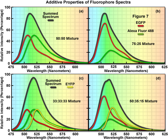
The additive properties of fluorophore spectra are examined theoretically in Figure 7(a) and 7(b) for a mixture of two different, but highly overlapping fluorophores. Similarly, in Figure 7(c) and 7(d) a more complex mixture containing three overlapping fluorophores is examined. The black curves in Figure 7(a)-7(d) represent the sum of two or three component fluorophore spectra. EGFP and Alexa Fluor 488, two probes that emit in the cyan-green spectral region, are shown in red and green in Figure 7(a) and 7(b) according to the following proportions: Figure 7(a), 50:50 and Figure 7(b), 75:25. Although these are examples of only two combinations, the summed spectrum can easily be predicted for every possible fluorophore combination. Likewise, in Figure 7(c), EGFP, Alexa Fluor 488, and EYFP are illustrated in an equal (33:33:33) mixture to produce a summed spectrum. In Figure 7(d), the same fluorophores are mixed in proportions of 50:35:15. Note the changes to the summed spectra profiles as the component fluorophore mixture is altered.
In order to determine the spectral content of each pixel in an image, the simplest approach would be to match the summed spectrum from that pixel with all possible sum combinations from a library, similar to what investigators undertake when they are matching a fingerprint with a database. For example, if the measured summed spectrum was a very close match to the black curve presented in the first panel in Figure 7, it could be concluded that the two fluorophores were evenly mixed in that pixel. Likewise, if the summed spectrum matched the black curve in the second panel (Figure 7(b)), it would indicate that the pixel contained 75 percent of one fluorophore and 25 percent of the other. In review, linear unmixing is a straightforward technique that compares a matrix representing the summed spectra measured in an image against a library of predicted spectra according to the best-fit parameters mandated by the software. After the contribution of each spectral component is determined, the lambda stack can then be segregated into individual images for each fluorophore. Thus, the intensity of an individual pixel in the unmixed spectral image represents the total measured pixel intensity multiplied by the proportion of each fluorophore spectra in that pixel. The result of linear unmixing is conversion of a lambda stack into individual images (see Figure 1) representing the signal profile for each fluorophore.
Alternative approaches to spectral unmixing of fluorescence emission have also emerged and should be considered for small datasets consisting of only a few spectral channels. One of the simplest relies on the colocalization scatterplot strategy that plots the intensity values of a pixel in different spectral channels on separate axes of a Cartesian coordinate system (termed Adaptive Dye Separation). The characteristic spectral signatures of fluorophores in the specimen are then determined by cluster analysis through the fitting of lines in pixel regions where only a single fluorophore predominates. Thus, spectral scans are not required as the technique takes advantage of the fact that spectral characteristics are present in a standard multicolor image (provided more than two or more fluorescent probes are not highly colocalized). Separation of spectra is accomplished by determining the distribution angles of individual probes and orthogonalizing the scatterplot into different channels (in effect, the stretching each fluorophore cluster and relocating it to different axes on the plot). The most significant advantage of this technique is that it does not require prior knowledge of the different fluorophore spectra because the spatial distributions are determined by line fitting after images are acquired. However, scatterplot analysis becomes increasingly complex when more than two fluorophores are analyzed and the methodology is only reliable if significant levels of emission from a single probe are present in a given pixel without contamination by other probes.
Another solution to spectral unmixing entails a simple channel subtraction approach, but this technique is applicable only in situations where at least one fluorophore channel does not have mixed contribution from other fluorophores in the specimen. Furthermore, subtraction is really only a viable alternative when the specimen is labeled with a limited number of probes (usually two or three). In practice, the microscope must be configured so that the contribution of one fluorophore (F1) in the detection channel for the second fluorophore (F2) can be unambiguously determined and expressed as a normalized value (R). Then the contribution of the second fluorophore minus that of the first can be obtained by simple subtraction using information from the first channel:
R = (F1ch2 / F1ch1)
F2 = Ch2 - (R Ch1)
For investigations using multiple fluorophores, the condition of having at least one spectral channel limited to contain intensity values from only a single fluorophore (without any contribution from others) must be defined both at the beginning of the calculation and again after the subtraction of each fluorophore, which severely limits this methodology to only a small subset of those experiments that can be readily solved with linear unmixing algorithms. As a result, many two-fluorophore combinations cannot be analyzed by the subtraction method, and the use of more than two fluorophores often requires stringent filter specifications that limit the available signal level. Further hampering the channel subtraction approach is the fact that signal from a fluorophore detected in other channels (and subtracted) is not utilized in the final calculations. In contrast, linear unmixing analyzes the total signal from all channels and redistributes the signal levels according to the individual contributions from each fluorophore. The result is a much brighter image than is possible with subtraction techniques. Generally, channel subtraction should be limited to situations where a spectral imaging instrument is unavailable or when a highly defined system that responds well to the method is repeatedly studied.
Spectral unmixing is an important and emerging technique that is increasingly being applied to brightfield measurements conducted on pathological specimens stained with absorbing dyes (such as eosin and hematoxylin). Such analysis employs algorithms similar to the linear unmixing described above, but takes into account specific factors that apply to absorption rather than emission spectra. A complicating feature of brightfield analysis is that the absorption registered for each pixel must be calculated from the measured transmission data. Fortunately, in most cases the absorption spectrum of a synthetic dye molecule is linearly dependent on the concentration, which diminishes the complexity of spectral measurements. Similar to the case for fluorescence, when a specimen contains several absorbing stains, the transmission spectrum acquires a complex structure with an overall absorbance profile that combines the different dyes:
A(λ) = Σi εi(λ) Ci li
where A is the absorbance of species (i), C is the concentration, and l is the specimen optical pathlength (usually measured in micrometers for thin sections of stained tissue). The preliminary step of the calculation is to determine the optical density (OD) of each species from the measured transmission:
OD = log10{Ii(λ) / Io(λ)}
In situations where the signal level is low, conversion of transmission data to optical density can result in the introduction of a significant level of noise. Under these circumstances, excluding the spectral tails can aid in the final analysis. Similar to the case for linear unmixing of fluorescent species, if the absorption spectra for the different dyes present in a specimen can be independently determined, it should be possible to calculate the concentration of each stain in every pixel of the image. Caution should be exercised in examining certain brightfield specimens due to the fact that some stains, such as diaminobenzidine, are actually scattering polymers that do not absorb light. As a consequence, the linearity assumption described above is not valid and the quantitative analysis of stains in these specimens may not yield reasonable values. Another artifact that can occur is a complex interaction between histological stains in tissue sections that hampers the isolation of individual component spectra. Often in these cases, a similarity mapping algorithm, which is based on information provided by the specimen itself (or from similar specimens), can be used to aid in the identification of spectral components.
Commercial instruments equipped for spectral imaging and linear unmixing bundle the hardware and software into an integrated package that, in most cases, is user-friendly and highly functional. There are, however, several practical considerations that will assist in ensuring the greatest potential for success in real-world investigations. Perhaps the most important aspect is to carefully gather reference spectra for all fluorophores that faithfully represent the spectra likely to be obtained from the test specimen. In this regard, all controls must (without deviation) be imaged under identical conditions. Pixel saturation and high background noise should be avoided, and autofluorescence should be taken into consideration as a component spectrum in cases where it cannot be eliminated. In addition, unwanted signal from laser lines and mounting media discontinuities can affect linear unmixing results. Finally, low signal levels arising from dispersing the emission signal over a broad spectral range can adversely affect the results of quantitative experiments. Whenever possible, fluorophore concentrations (or at least signal levels) should be as closely matched as possible to ensure optimum results.
The microscope optical train components (mirrors, lenses, filters, beamsplitters) will impose a considerable amount of bias on reference and test measurements, so collecting spectra from other instruments is unwise and will no doubt lead to errors. In order to avoid pitfalls, reference spectra should be acquired in exactly the same manner as the lambda stack, including using the same objective, pinhole diameter, offset, amplifier gain, photomultiplier voltage (not necessary when the gain responses are calibrated), wavelength range, dichromatic mirror, laser power, pixel dwell time, specimen mounting medium, coverslips, and immersion oil. The best approach is to determine the imaging parameters for the lambda stack first, and then acquire reference spectra under identical conditions. In specimens that exhibit considerable spatial separation of the fluorophores under consideration, it might be possible to chose non-overlapping regions from within the lambda stack itself for analysis.
Spectral Imaging Applications
Spectral imaging coupled with linear unmixing is becoming an increasing popular tool to solve a number of problems in research areas as diverse as spectral karyotyping, immunofluorescence, live-cell imaging, drug discovery, and tissue pathology. The spectral information provided by this technique enables investigators to detect and differentiate between a wide variety of absorbing dyes and fluorophores, even in situations where a significant degree of spectral overlap occurs. Such a tool opens the door to virtually unlimited use of mixed labels for quantitative analysis in a wide variety of specimens. Furthermore, the highly refined spectral information available with linear unmixing can be employed to distinguish between artifacts, such as autofluorescence and refractive index fluctuations in mounting media, and the sought after contributions of legitimate signal from probes that have successfully hit their intended target. Spectral imaging is also useful as a monitor for dynamic processes, which often feature temporal variations in contrast and altered spectral profiles of interacting labels. Virtually any modern widefield or confocal microscope can be readily adapted to acquire spectral image data, and many commercial solutions have been available for several years and have proven track records. The software analysis of spectral data, in many cases, has become seamlessly integrated with the host instrumentation, but aftermarket products are also quite useful for various aspects of data analysis and are often much cheaper. It should be borne in mind, however, that integrated software and hardware packages, such as those spectral imaging confocal microscopes offered by the major manufacturers, benefit from the advantage of access to the instrument meta data (such as photomultiplier calibration curves necessary for error plotting) that is generally lacking in aftermarket products.
Perhaps the most widespread application of spectral imaging currently in use today is spectral karyotyping for the analysis of chromosomes using widefield fluorescence in situ hybridization (FISH) methodology. In most cases, fluorescence karyotyping employs in excess of five different probes to individually label the entire set of metaphase chromosomes in human or other mammalian cells. Typically, each chromosome is labeled with a different combination of synthetic fluorophores, which can be derived from a large variety of common probes including the cyanine (Cy) dyes, fluorescein, Atto dyes, rhodamine, and Alexa Fluors. There are 31 possible two-dye combinations when five fluorophores are used so that enough variability is on hand to specifically label each of the 24 human chromosomes. After linear unmixing, the resulting spectral image is segmented, and each pixel then classified based on its spectrum before being compared to a library of fluorophore reference spectra. Modern instrumentation provides sufficiently high specificity to enable successful classification in a majority of experiments, even when applied to difficult specimens.
Autofluorescence poses significant problems in all phases of fluorescence microscopy and whole body imaging, particularly when specimens have been prepared using paraformaldehyde or skin components are being imaged. Many fixation procedures dramatically increase autofluorescence levels to the point that they often overwhelm the signal from fluorophores used to stain specific regions in the adherent cells or tissue. Plant and neural tissues also tend to exhibit a high degree of intrinsic autofluorescence and, in addition, the transfection reagents commonly used to mediate fluorescent protein vector DNA entry into mammalian cells can increase autofluorescence signal. Spectral imaging and linear unmixing can be employed to treat autofluorescence as a separate fluorophore having a distinct emission fingerprint that can be resolved from the signals of interest. In this manner, the unwanted autofluorescence signal can be dramatically reduced or eliminated completely in the final images. Note that autofluorescence is decreased when imaging at longer wavelengths (greater than 550 nanometers) so that judicious choice of fluorophores in the red, far-red, or near-infrared spectral regions can also be an effective remedy to minimize this artifact.
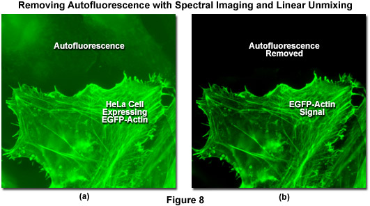
Illustrated in Figure 8 is the removal of autofluorescence in a transiently transfected culture of HeLa cells expressing a fusion of EGFP to human beta-actin. Autofluorescence arises from a combination of high background signal produced by the lipid-based transfection reagent as well as biomolecules naturally present in cells that fluoresce upon exposure to illumination in the cyan spectral region. In this case, the autofluorescence in the upper section of Figure 8(a) was treated as an additional fluorophore and subtracted from the spectrally unmixed image in Figure 8(b). Autofluorescence is often a problem when imaging fluorescent proteins (in both fixed and live cell preparations) due to the relatively low brightness exhibited by these probes when compared to synthetics such as Alexa Fluor 488. The brightest fluorescent proteins in the orange through red spectral regions, including tandem-dimer Tomato (tdTomato) and mOrange, can be readily imaged without far less concern for autofluorescence, due both to the exceptional probe brightness and to the decreased excitation of endogenous fluorophores by longer wavelength illumination.
Aside from its ability to separate the emission fingerprints of closely overlapping fluorophores in multicolor fixed and live-cell imaging, spectral imaging is also useful to help resolve and quantitate the complex signals often encountered in FRET investigations. In most cases, the donor and acceptor signals exhibit significant overlap, thus rendering the separation of these individual contributions one of the most significant difficulties in determining FRET efficiency. In spectral imaging of FRET specimens (usually conducted on live cells expressing fluorescent proteins), the entire spectral response from both fluorophores is measured. Although spectral imaging is capable of unambiguously detecting donor and acceptor emission signals without bleed-through, the technique is incapable of distinguishing between acceptor emission generated through energy transfer and emission signal that originates from direct excitation of the acceptor. Therefore, the proper controls must always be included in these experiments. In addition, spectral imaging for FRET is generally used in combination with acceptor photobleaching techniques as a cross-check. In cases where spectral imaging is used to examine dynamic FRET changes in genetically-encoded biosensors, such as calcium-sensitive cameleons, the use of controls is less important.
Spectral imaging and linear unmixing is also commonly applied to the examination of brightfield specimens stained with absorbing dyes that can exhibit significant spectral overlap. In this case, the signal is usually very bright (high signal-to-noise ratio) and photobleaching is so minimal as to not be a problem. However, synthetic dye mixtures used to stain tissues often have a very complex spectrum that is dependent upon the number of dyes used in the specimen. When more than three dyes are used, the specimens often acquire a brownish, murky appearance. Spectral imaging enables the analysis and separation of multiple absorbing dyes in brightfield mode to generate a series of single-color images that mimic how the specimen would appear with only a single stain. The set of images can then be correlated to determine colocalization of dyes within specific structures. Among the artifacts often encountered in spectral imaging of brightfield specimens is changes to dye absorption spectra that occur due to local environmental conditions. Overstaining is another common problem that complicates spectral imaging of these specimens.
Conclusions
Spectral imaging coupled to linear unmixing techniques is becoming an important staple in the microscopist's toolbox, particularly when applied to the reduction of autofluorescence in live-cell imaging and for FRET investigations. Instruments equipped for spectral imaging are becoming increasingly popular and many confocal microscopes now offer this capability. Widefield fluorescence and brightfield microscopy are also being used more frequently for resolving complex fluorophore and absorbing dye mixtures, a trend that should continue into the future.
Contributing Authors
Mary E. Dickinson - Department of Molecular Physiology and Biophysics, One Baylor Plaza BCM 335, Baylor College of Medicine, Houston, Texas, 77030.
Michael W. Davidson - National High Magnetic Field Laboratory, 1800 East Paul Dirac Dr., The Florida State University, Tallahassee, Florida, 32310.