


The process of linear unmixing of data obtained from spectral imaging is a mechanism for matching the spectral variations in the lambda stack with the known spectral variations for the fluorophores present in the specimen. For each pixel in the image, the fluorescence intensity of colocalized fluorophores having overlapping emission spectra will be the sum of the intensity for each individual fluorophore. This interactive tutorial explores how multiple spectra can be added to produce a composite emission spectrum similar to those encountered in spectral imaging of specimens labeled with multiple fluorophores.

The tutorial initializes with a summed spectrum (black curve) from a 50:50 mixture of EGFP (red curve) and Alexa Fluor 488 (green curve) being presented in the spectral window. The intensity contribution of each probe (Ii(λ)) to the total intensity as a function of wavelength (I(λ)) is presented below the graph. In order to operate the tutorial, use the sliders to adjust the contribution of Fluorophore A and Fluorophore B between the ranges of zero and 100 percent. The pull-down menus enable selection of different fluorophores in the same color region. Selecting a third fluorophore from the lower pull-down menu (Fluorophore C) adds the ability to examine summed spectra having three components. The contribution of a particular fluorophore in the three component model can be locked by clicking on the padlock icon to the left of the slider. Once a single fluorophore is locked, the contribution of the remaining two fluorophores can be altered.
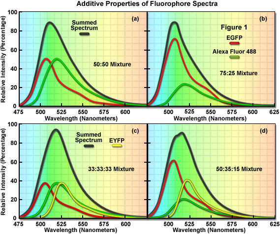
The additive properties of fluorophore spectra are examined theoretically in Figure 1(a) and 1(b) for a mixture of two different, but highly overlapping fluorophores. Similarly, in Figure 1(c) and 1(d) a more complex mixture containing three overlapping fluorophores is examined. The black curves in Figure 1(a)-1(d) represent the sum of two or three component fluorophore spectra. EGFP and Alexa Fluor 488, two probes that emit in the cyan-green spectral region, are shown in red and green in Figure 7(a) and 7(b) according to the following proportions: Figure 1(a), 50:50 and Figure 1(b), 75:25. Although these are examples of only two combinations, the summed spectrum can easily be predicted for every possible fluorophore combination. Likewise, in Figure 1(c), EGFP, Alexa Fluor 488, and EYFP are illustrated in an equal (33:33:33) mixture to produce a summed spectrum. In Figure 1(d), the same fluorophores are mixed in proportions of 50:35:15. Note the changes to the summed spectra profiles as the component fluorophore mixture is altered.
In order to determine the spectral content of each pixel in an image, the simplest approach would be to match the summed spectrum from that pixel with all possible sum combinations from a library, similar to what investigators undertake when they are matching a fingerprint with a database. For example, if the measured summed spectrum was a very close match to the black curve presented in the first panel in Figure 1, it could be concluded that the two fluorophores were evenly mixed in that pixel. Likewise, if the summed spectrum matched the black curve in the second panel (Figure 1(b)), it would indicate that the pixel contained 75 percent of one fluorophore and 25 percent of the other. In review, linear unmixing is a straightforward technique that compares a matrix representing the summed spectra measured in an image against a library of predicted spectra according to the best-fit parameters mandated by the software. After the contribution of each spectral component is determined, the lambda stack can then be segregated into individual images for each fluorophore. Thus, the intensity of an individual pixel in the unmixed spectral image represents the total measured pixel intensity multiplied by the proportion of each fluorophore spectra in that pixel. The result of linear unmixing is conversion of a lambda stack into individual images representing the signal profile for each fluorophore.
Contributing Authors
Adam M. Rainey and Michael W. Davidson - National High Magnetic Field Laboratory, 1800 East Paul Dirac Dr., The Florida State University, Tallahassee, Florida, 32310.