


Introduction
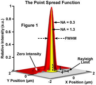
The ideal point spread function (PSF) is the three-dimensional diffraction pattern of light emitted from an infinitely small point source in the specimen and transmitted to the image plane through a high numerical aperture (NA) objective. It is considered to be the fundamental unit of an image in theoretical models of image formation. When light is emitted from such a point object, a fraction of it is collected by the objective and focused at a corresponding point in the image plane. However, the objective lens does not focus the emitted light to an infinitely small point in the image plane. Rather, light waves converge and interfere at the focal point to produce a diffraction pattern of concentric rings of light surrounding a central, bright disk, when viewed in the x-y plane. The radius of disk is determined by the NA, thus the resolving power of an objective lens can be evaluated by measuring the size of the Airy disk (named after George Biddell Airy). The image of the diffraction pattern can be represented as an intensity distribution as shown in Figure 1. The bright central portion of the Airy disk and concentric rings of light correspond to intensity peaks in the distribution. In Figure 1, relative intensity is plotted as a function of spatial position for PSFs from objectives having numerical apertures of 0.3 and 1.3. The full-width at half maximum (FWHM) is indicated for the lower NA objective along with the Rayleigh limit.
In a perfect lens with no spherical aberration the diffraction pattern at the paraxial (perfect) focal point is both symmetrical and periodic in the lateral and axial planes. When viewed in either axial meridian (x-y or y-z) the diffraction image can have various shapes depending on the type of instrument used (i.e. widefield, confocal, or multiphoton) but is often hourglass or football-shaped. The point spread function is generated from the z series of optical sections and can be used to evaluate the axial resolution. As with lateral resolution, the minimum distance the diffraction images of two points can approach each other and still be resolved is the axial resolution limit. The image data are represented as an axial intensity distribution in which the minimum resolvable distance is defined as the first minimum of the distribution curve.
The PSF is often measured using a fluorescent bead embedded in a gel that approximates an infinitely small point object in a homogeneous medium. However, thick biological specimens are far from homogeneous. Differing refractive indices of cell materials, tissues, or structures in and around the focal plane can diffract light and result in a PSF that deviates from design specification, fluorescent bead determination or the calculated, theoretical PSF. A number of approaches to this problem have been suggested including comparison of theoretical and empirical PSFs, embedding a fluorescent microsphere in the specimen or measuring the PSF using a subresolution object native to the specimen.
The PSF is valuable not only for determining the resolution performance of different objectives and imaging systems, but also as a fundamental concept used in deconvolution. Deconvolution is a mathematical transformation of image data that reduces out of focus light or blur. Blurring is a significant source of image degradation in three-dimensional (3D) widefield fluorescence microscopy. It is nonrandom and arises within the optical train and specimen, largely as a result of diffraction. A computational model of the blurring process, based on the convolution of a point object and its PSF, can be used to deconvolve or reassign out of focus light back to its point of origin. Deconvolution is used most often in 3D widefield imaging. However, even images produced with confocal, spinning disk, and multiphoton microscopes can be improved using image restoration algorithms.
Image formation begins with the assumptions that the process is linear and shift invariant. If the sum of the images of two discrete objects is identical to the image of the combined object, the condition of linearity is met, providing the detector is linear, and quenching and self-absorption by fluorophores is minimized. When the process is shift invariant, the image of a point object will be the same everywhere in the field of view. Shift invariance is an ideal condition that no real imaging system meets. Nevertheless, the assumption is reasonable for high quality research instruments.
Convolution mathematically describes the relationship between the specimen and its optical image. Each point object in the specimen is represented by a blurred image of the object (the PSF) in the image plane. An image consists of the sum of each PSF multiplied by a function representing the intensity of light emanating from its corresponding point object:
i(x) =  o(x - x') × psf(x')dx'(1)
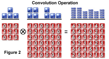
A pixel blurring kernel is used in convolution operations to enhance the contrast of edges and boundaries and the higher spatial frequencies in an image. Figure 2 illustrates the convolution operation using a 3 x 3 kernel to convolve a 6 x 6 pixel object. Above the arrays in Figure 2 are profiles demonstrating the maximum projection of the two-dimensional grids when viewed from above.
An image is a convolution of the object and the PSF and can be symbolically represented as follows:
image(r) = object(r) ⊗ psf(r)(2)
where the image, object, and PSF are denoted as functions of position (r) or an x, y, z and t (time) coordinate. The Fourier transform shows the frequency and amplitude relationship between the object and point spread function, converting the space variant function to a frequency variant function. Because convolution in the spatial domain is equal to multiplication in the frequency domain, convolutions are more easily manipulated by taking their Fourier transform (F).
F{i(x,y,z,t)} = F{o(x,y,z,t)} × F{psf(x,y,z,t)}(3)
In the spatial domain described by the PSF, a specimen is a collection of point objects and the image is a superposition or sum of point source images. The frequency domain is characterized by the optical transfer function (OTF). The OTF is the Fourier transform of the PSF and describes how spatial frequency is affected by blurring. In the frequency domain, the specimen is equivalent to the superposition of sine and cosine functions, and the image consists of the sum of weighted sine and cosine functions. The Fourier transform further simplifies the representation of the convolved object and image such that the transform of the image is equal to the specimen multiplied by the OTF. The microscope passes low frequency (large, smooth) components best, intermediate frequencies are attenuated, and high frequencies greater than 2NA/λ are excluded. Deconvolution algorithms are therefore required to augment high spatial frequency components.
Theoretically, it should be possible to reverse the convolution of object and PSF by taking the inverse of the Fourier transformed functions. However, deconvolution increases noise, which exists at all frequencies in the image. Beyond half the Nyquist sampling frequency no useful data are retained, but noise is nevertheless amplified by deconvolution. Contemporary image restoration algorithms use additional assumptions about the object such as smoothness or non-negative value and incorporate information about the noise process to avoid some of the noise related limitations.
Deconvolution algorithms are of two basic types. Deblurring algorithms use the PSF to estimate blur then subtract it by applying the computational operation to each optical section in a z-series. Algorithms of this type include nearest neighbor, multi neighbor, no neighbor, and unsharp masking. The more commonly used nearest neighbor algorithm estimates and subtracts blur from z sections above and below the section to be sharpened. While these run quickly and use less computer memory, they don't account for cross-talk between distant optical sections. Deblurring algorithms may decrease the signal-to-noise ratio (SNR) by adding noise from multiple planes. Images of objects whose PSFs overlap in the paraxial plane can often be sharpened by deconvolution, however, at the cost of displacement of the PSF. Deblurring algorithms introduce artifacts or changes in the relative intensities of pixels and thus cannot be used for morphometric measurements, quantitative intensity determinations or intensity ratio calculations.
Image restoration algorithms use a variety of methods to reassign out-of-focus light to its proper position in the image. These include inverse filter types such as Wiener deconvolution or linear least squares, constrained iterative methods such as Jansson van Cittert, statistical image restoration, and blind deconvolution. Constrained deconvolution imposes limitations by excluding non-negative pixels and placing finite limits on size or fluorescent emission, for example. An estimation of the specimen is made and an image calculated and compared to the recorded image. If the estimation is correct, constraints are enforced and unwanted features are excluded. This process is convenient to iterative methods that repeat the constraint algorithm many times. The Jansson van Cittert algorithm predicts an image, applies constraints, and calculates a weighted error that is used to produce a new image estimate for multiple iterations. This algorithm has been effective in reducing high frequency noise.
Blind deconvolution does not use a calculated or measured PSF but rather, calculates the most probable combination of object and PSF for a given data set. This method is also iterative and has been successfully applied to confocal images. Actual PSFs are degraded by the varying refractive indices of heterogeneous specimens. In laser scanning confocal microscopy, where light levels are typically low, this effect is compounded. Blind deconvolution reconstructs both the PSF and the deconvolved image data. Compared with deblurring algorithms, image restoration methods are faster, frequently result in better image quality, and are amenable to quantitative analysis.
Deconvolution performs its operations using floating point numbers and consequently, uses large amounts of computing power. Four bytes per pixel are required, which translates to 64 Mb for a 512 x 512 x 64 image stack. Deconvolution is also CPU intensive, and large data sets with numerous iterations may take several hours to produce a fully restored image depending on processor speed. Choosing an appropriate deconvolution algorithm involves determining a delicate balance of resolution, processing speed, and noise that is correct for a particular application.
Contributing Author
Rudi Rottenfusser - Zeiss Microscopy Consultant, 46 Landfall, Falmouth, Massachusetts, 02540.
Erin E. Wilson and Michael W. Davidson - National High Magnetic Field Laboratory, 1800 East Paul Dirac Dr., The Florida State University, Tallahassee, Florida, 32310.